I carried out this analysis a few months ago for one of the modules of the Sports Data Course “Statistics and Mathematics applied to sport with R”.
The purpose of this exercise is to make a comparison between two different clustering models, one non-hierarchical and the other one hierarchical.
The data used are selected by me and obtained from the Fbref website, based on offensive metrics for the 2022-2023 season.
SAMPLE SELECTION
Before doing any step in the algorithm, we have to select the sample with all the data we want to be taken in consideration. This process is important, because depending on what we choose, the clustering result will vary.
As the data we have corresponds exclusively to offensive metrics, we will restrict the sample by position, by minutes played, by certain leagues and by a certain number of metrics:
- Position: Strikers.
- Minutes played: Same or more than 2,500 minutes played.
- Leagues: La Liga, Premier League, Bundesliga and Ligue 1.
- Selected metrics: Goals, xG, xG excluding penalties, shots, shots on target, percentage of shots on target and goals per shots (all metrics always given per 90 minutes).
STANDARDISATION AND OUTLIERS
STANDARDISATION
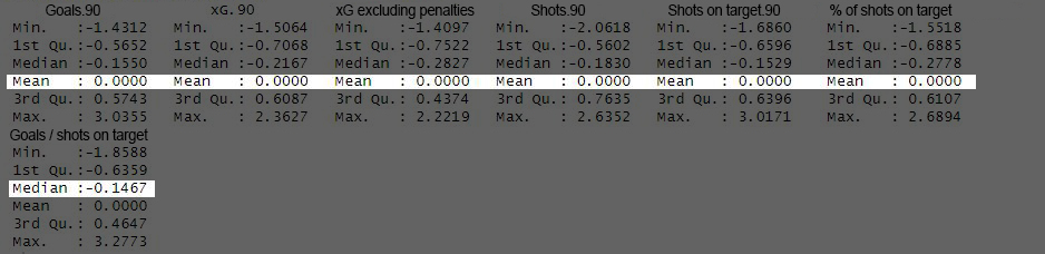
Once the final sample is ready, the next step is to standardise these variables to avoid one variable being more important than others because they are measured in different magnitudes.
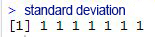
This is achieved by making all the variables mean equal to 0 and the standard deviation equal to 1.
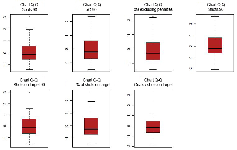
OUTLIERS
Identifying outliers can be crucial in determining distances, as they can have a strong influence on our analysis.
EVALUATION OF CLUSTERING TENDENCY
The last step before starting the clustering analysis will be to evaluate the sample to see if the data are groupable, in other words, to see if the players in the dataset have certain similarities and certain differences which allow a good segmentation of the data.
This is achieved with the Hopkins statistic:
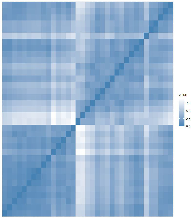
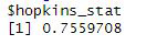
The Hopkins Statistic is a value between 0 and 1, and the closer the value is to 1, better to do clustering (in this case, as the result is 0.7559708, it means that it is optimal for clustering).
NON-HIERARCHICAL CLUSTERING ANALYSIS: K-MEANS
It’s time to apply the clustering algorithm, and we will start with the non-hierarchical K-Means method.
- As it is an unsupervised algorithm, we must tell the algorithm how many clusters we are interested in having.
- How do you determine the optimal number of clusters? A good way is to apply the “Elbow Rule”.
- The curve it makes is the sum of squared errors within the clusters and the point where the curve tends to stabilise is chosen.
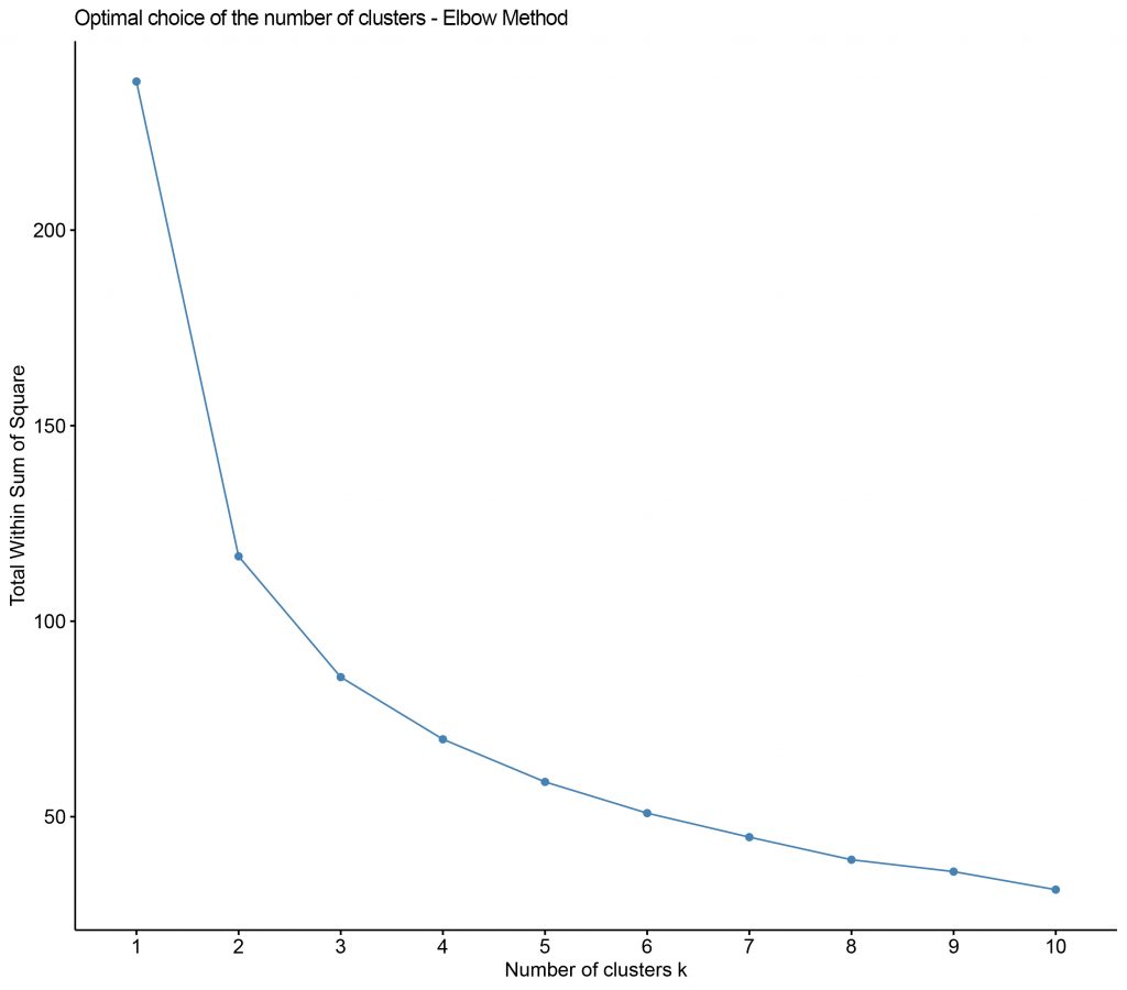
We see that according to the elbow rule we can determine 3 as the optimal number of clusters.
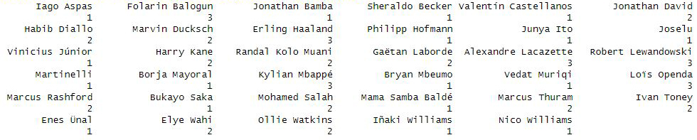
Now, the clustering algorithm is applied and we obtain the name of each player in the sample with the cluster number to which they correspond:
If I apply principal component analysis (PCA), using only the first two dimensions (which are the ones with the most information), we can see this information represented in a chart:
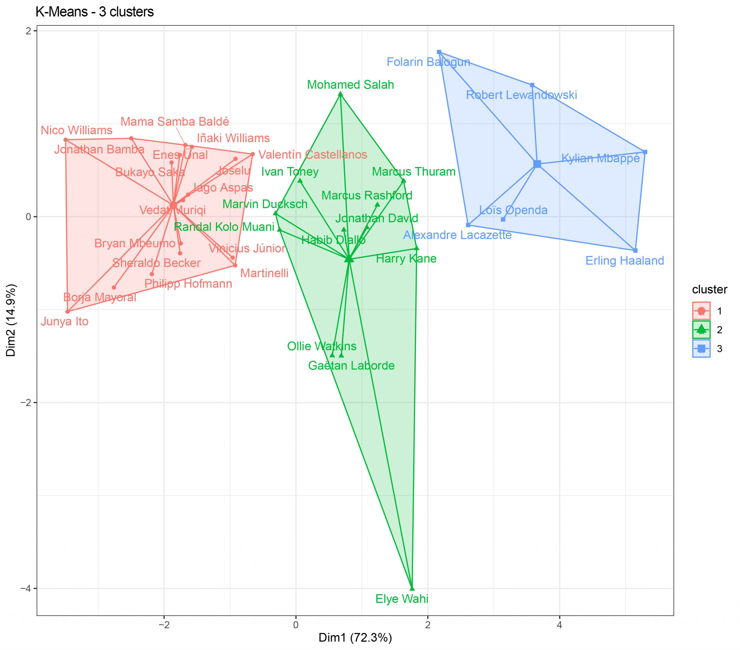
- We see 3 clusters, number 1, formed by players who play mostly in medium-low quality teams, where their scoring statistics may suffer (the top scorer in this group is Joselu, with 16 goals).
- In cluster 2 we see players with superior scoring statistics and who mostly play in top teams, but who haven’t had a season at the level expected, such as Salah (19 goals, far from his usual records), Marcus Rashford (17 goals) or Harry Kane (30 goals and a great season despite his team’s poor performance).
- In the last cluster we see, among others, the top scorers in La Liga (Lewandowski, 23 goals), Ligue 1 (Mbappé, 29 goals) and Premier League (Haaland, 36 goals).
I could also select just a couple of variables that I consider important and make a scatter plot of them facing each other.
For example, I find it interesting to see who is the most effective striker, not the highest scorer, but the one who needs fewer shots to score more goals (always talking per 90 minutes):

- We can see that the clusters are well defined.
- Breaking down the information shown in the chart, we see that Haaland is by far the striker who has the best ratio between the shots he needs to take and the goals he scores, while, for example, the second world star, Mbappé, needs to shoot much more to score a goal.
- To compare Mbappé with the second top scorer in Ligue 1, the chart shows that although Mbappé scores more goals per ninety minutes, Lacazette is more effective in front of goal, needing fewer shots to score.
- But as in this chart we are talking about efficiency, let’s note that there are players in cluster 1, the group of the medium-low quality teams, who are also effective, such as Borja Mayoral or Nico Williams.
- It’s surprising that Vinícius is also in cluster 1, which indicates that despite having improved enormously in finishing in the last two seasons, he still needs to generate a lot of chances to score goals.
- Keeping all this in mind, we should keep in mind that the more shots on target, the harder it will be to maintain a high percentage of efficiency.
EVALUATION OF PARTITIONS
Finally, we are going to make an evaluation of the partitions we have made, that is, we are going to see how our three clusters are doing by applying the Silhouette method.
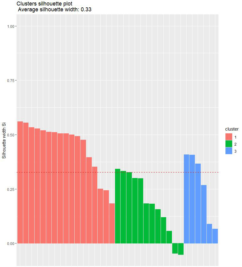
We see the players in each group:
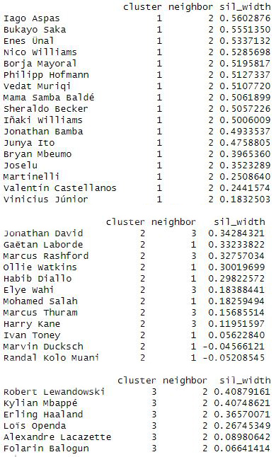
- Accessing each individual cluster we see that in cluster 2 we have Kolo Muani and Marvin Ducksch, who could be in another cluster if more were formed.
- In clusters 1 and 3 it seems that all players are well placed.
HIERARCHICAL CLUSTERING ANALYSIS
Once the NON-hierarchical K-means clustering process has been completed, we will contrast it with the hierarchical clustering method.
By loading different clustering methods (e.g. “Average” or “Complete”), the next step is to calculate the cophenetic distance with all these methods to find out which of them explains best the real distance between the players.
DENDOGRAM REPRESENTATION
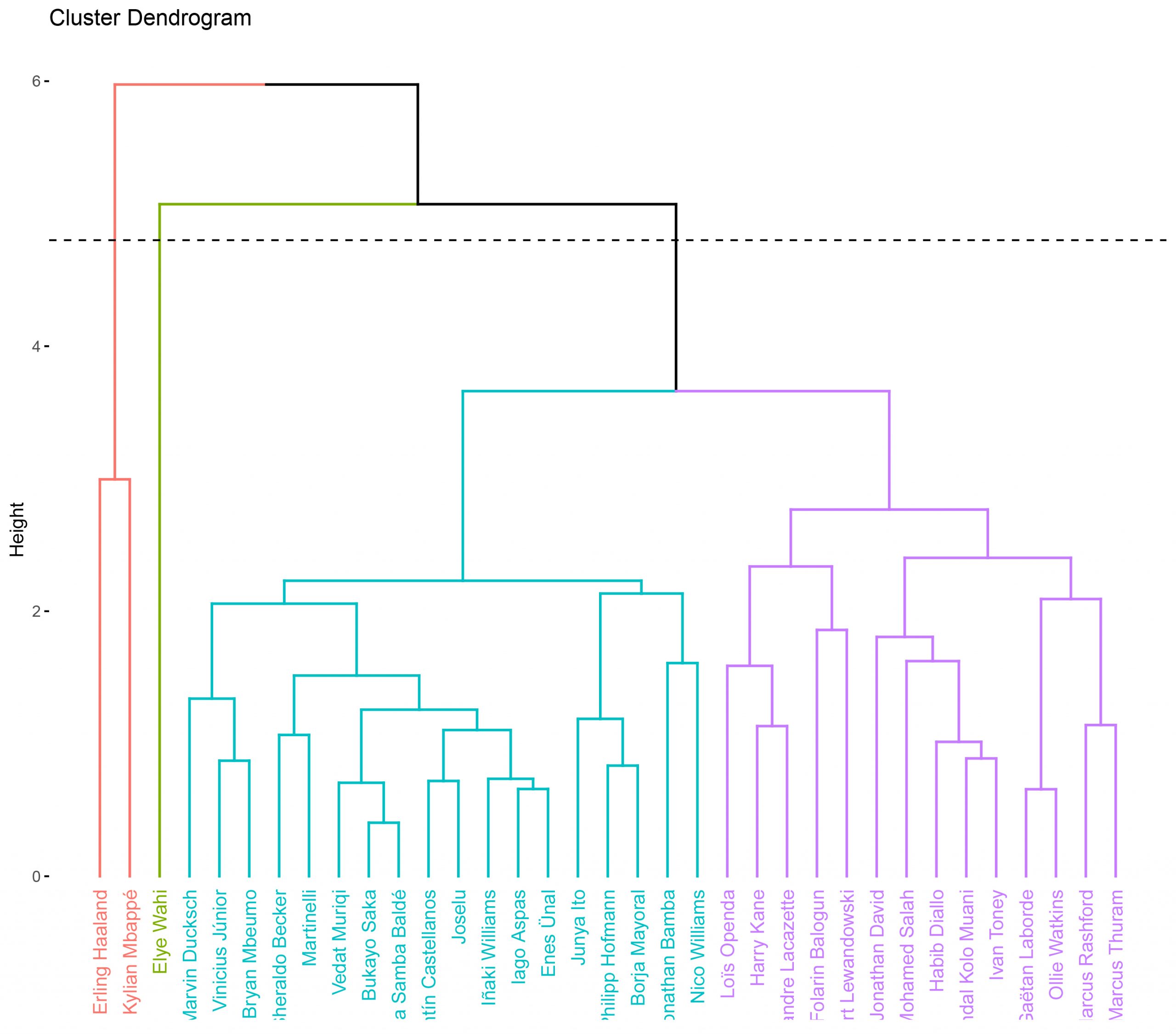
We are going to represent a dendogram and, according to the result obtained in the previous step in the calculation of the Cophenetic distance, we will use: Euclidean distance and the “Average” method.
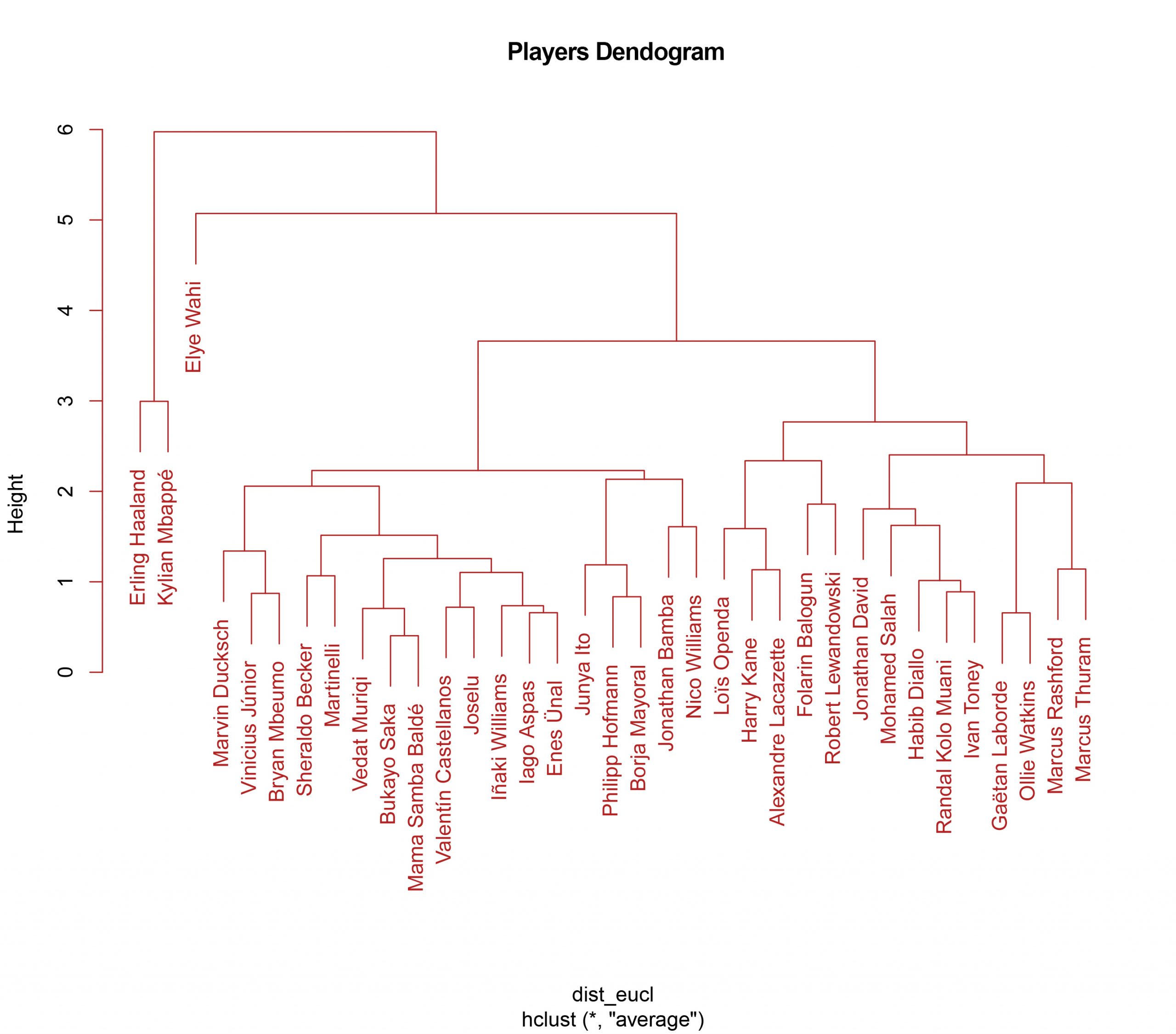
- We can see how we can already distinguish different groups or clusters.
- There are some players who are very differentiated, the “bosses”, Haaland and Mbappé, and we also see Elye Wahi separated from the rest, another young striker (20 years old) who has had a spectacular season with Montpellier, scoring 19 goals.
- Bukayo Saka of Arsenal and Mama Samba Baldé of Troyes seem to be the most similar players.
- We also see a lot of similarities between, for example, Celta’s Iago Aspas and Getafe’s Enes Ünal.
From this dendogram, I will generate another one indicating directly how many partitions I want (in this case, 4 partitions).
It can also be visualised using the two dimensions with PCA, as before in the K-Means visualisations:
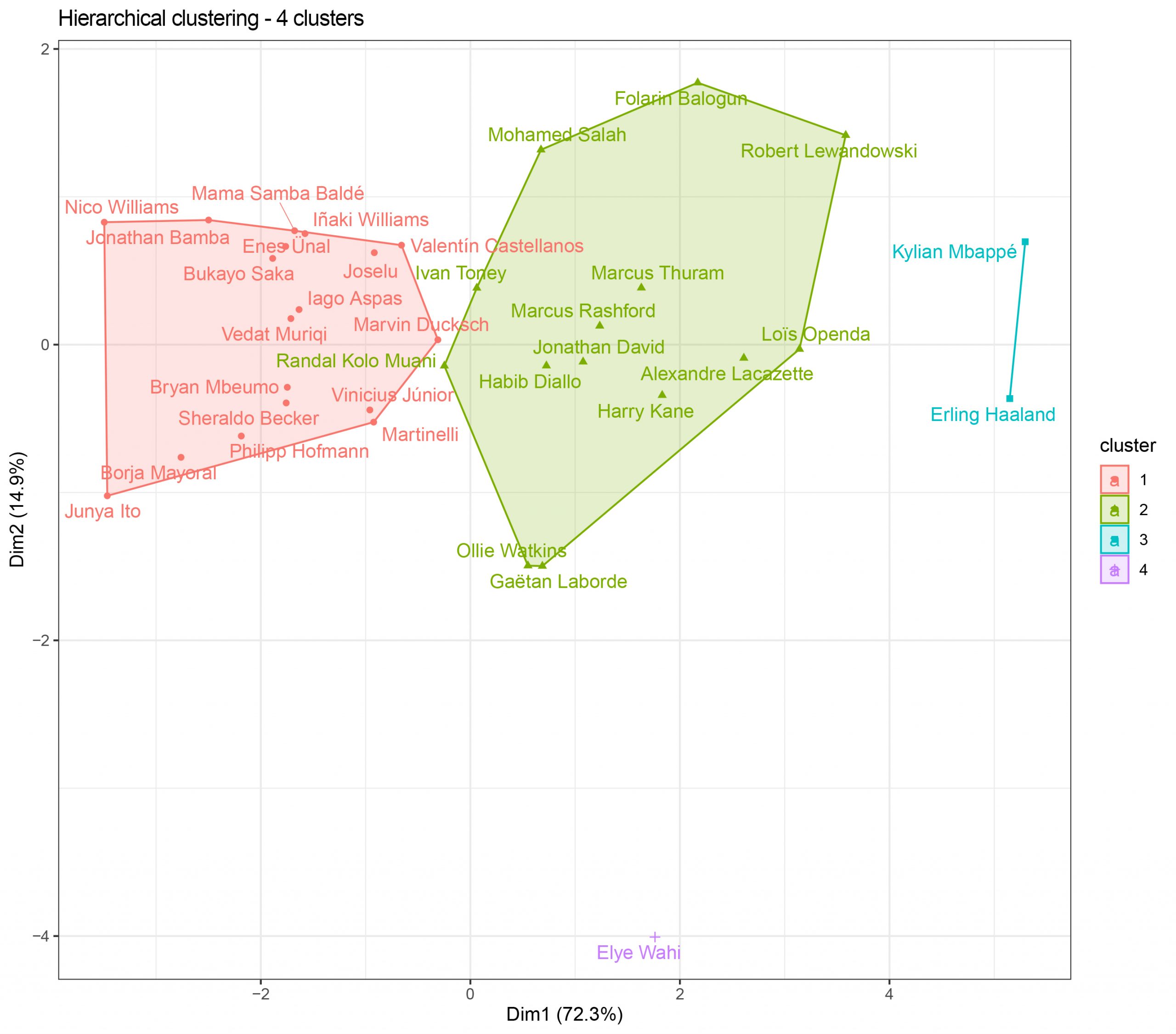
We see how with four clusters Elye Wahi remains as an independent cluster, while we have another cluster formed only by Haaland and Mbappé.
If we test with 3 clusters, which were chosen for K-Means…
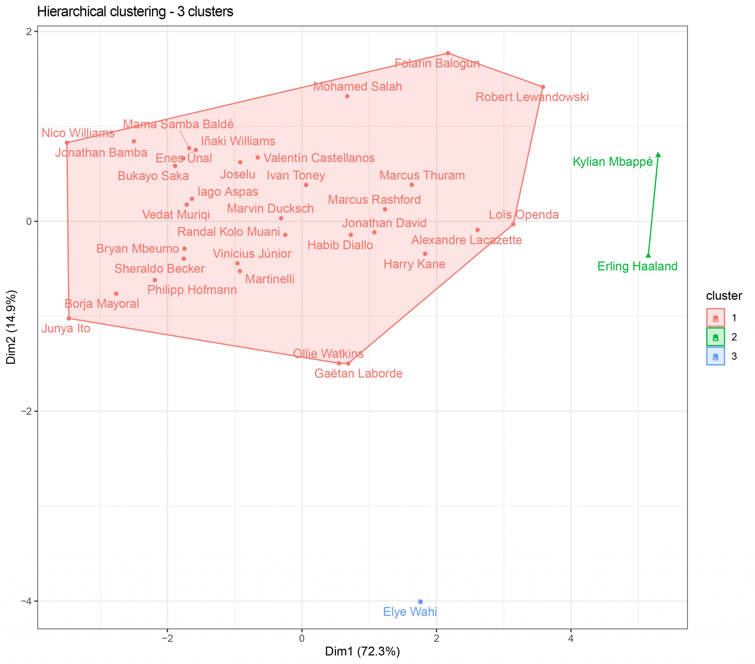
The result is not convincing… Clusters 1 and 2 have been merged and it doesn’t seem very realistic to have players like Junya Ito, Iñaki Williams or Mayoral in the same group with Harry Kane, Lewandowski or Rashford.
As with the K-Means method, I apply the Silhouette method to see if the observations or partitions are well classified.
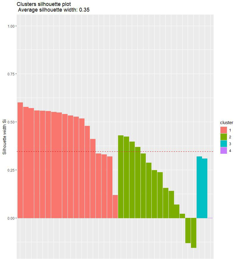
We see the players in each group:
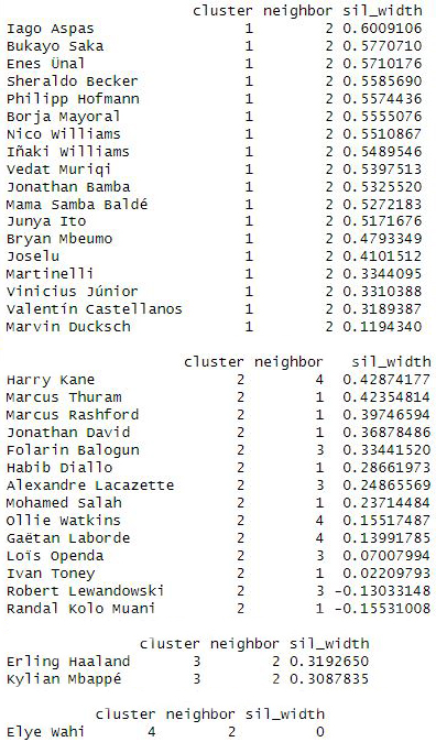
- Accessing each individual cluster we see that in cluster 1 the players seem to be well positioned.
- In cluster 2, Lewandowski and Kolo Muani could be in another cluster if more were to form.
- Cluster 3 is formed by Haaland and Mbappé.
- Cluster 4 is only formed by Elye Wahi.
DIFFERENCES BETWEEN MODELS
- In the hierarchical method we have added one more cluster and, while in K-Means Haaland and Mbappé were in the same group as other great strikers such as Lacazette or Lewandowski, here we have them alone as members of cluster 3.
- Elye Wahi was left as an independent cluster, while K-Means was in cluster 2.
- The silhouette method is very similar in both, 0.35 for hierarchical and 0.33 for K-Means.
Which method is better?… the answer is that one is not better than the other, it will depend on the data we have, so based on the data set used for this work, I would choose K-means, as it seems to me that it makes a more homogeneous separation.